Visualizing Mean Value Theorem in Mathematica

October 6, 2024

The mean value theorem is a surprising Calculus result that states for any function \(f\) differentiable on \((a,b)\)¹ there exists \(x\in(a,b)\) such that

\[f'(x)=\frac{f(b)-f(a)}{b-a}\] Here are three informal intuitions for what this means (all of them say the same thing in different ways):

1. Physical example. If you travel 60 miles in one hour, at some point you must have been traveling exactly 60 miles per hour.²
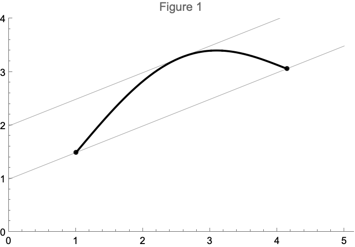
2. Geometric intuition. There exists a line tangent to \(f\) parallel to the line between the endpoints (i.e. parallel to the line between \((a, f(a))\) and \((b, f(b))\)). See figure 1 below for an illustration.
3. Algebraic intuition. There exists a point \(x\) at which instantaneous rate of change of \(f\) is equal to the average change of \(f\) on \([a,b]\).

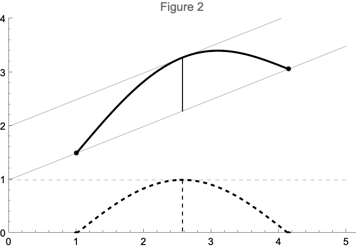
The proof is remarkably straightforward. You define a function \(h\) that maps values between \(a\) and \(b\) to a height from \(f\) to the line segment between the endpoints. This function \(h\) turns out to be differentiable, and hence has a maximum value (and hence there is a point \(a\) such that \(h'(a)=0\)). From there it's an easy algebraic transformation to demonstrate the mean value theorem is true. See figure 2 for an illustration.

Mathematica

I won't repeat the proof, but what I wanted to do is play with Mathematica to generate an interactive visualization of how the proof works (I generated above figures in Mathematica, but the final product has an interactive slider to make the proof more clear).

• Interactive visualization that you can play with is here.
• Mathematica notebook with the code is here.³

For tasks like this Mathematica is wonderful. Here I define a line at an angle, and another function \(f\) that adds a sine to it. Because the visualization is interactive \(s\) will allow the user to change the slope:

interpol[s_, a_, b_] := a + s*(b - a);

g[s_, x_] = interpol[s, 1/2, 0]*x + interpol[s, 1, 0];
f[s_, x_] = Sin[x - 1] + g[s, x];

These are symbolic definitions. We can plot them, take derivatives, integrate, and do all kinds of fancy computer algebra system operations. Here is an example. The vertical line in figure 2 comes down from the mean value of \(f\)-- i.e. a point on \(f\) where the tangent is parallel to the average change. In Mathematica code we can take the derivative of \(f\) (using Mathematica function D), and then solve (using Solve) for all values where the derivative is equal to mean value:

fD[a_] := D[f[s, x], x] /. x -> a;

avgSlope[s_] = (f[s, Pi + 1] - f[s, 1])/Pi;
meanPoint[s_] = 
  Solve[fD[x] == avgSlope[s] && x > 1 && x < Pi + 1, x];

This is the core of the code. Most of the rest of the code is plotting, which Mathematica does exceptionally well. I exported the plots to figures above using the Export function. Another notable function is Manipulate-- this is what makes the graph dynamic as the user drags a slider (by changing the variable s which the equations depend on). Finally I was able to publish the notebook in a few clicks, as well as publish the visualization itself using CloudDeploy. Instantaneous deployment of complex objects is very cool and useful.

Snags

There are a few things I don't like, but it's too early to say these are Mathematica's flaws (more likely it's my lack of familiarity):

• My sense is that the error messages aren't very good. I don't know how long it would take me to decipher them without ChatGPT.
• Cloud deployment is great, but on the web the slider is very laggy. That makes sense-- my code is symbolically solving for a particular value of a derivative, and I wouldn't expect Mathematica to implement all this in JavaScript. That means on the desktop client everything is instant, but on the web everything gets evaluated on the server. I could maybe restructure the code to not run the server-side solver with every slider drag, but it's not obvious how to do this.
• Mathematica supports embedding cloud objects in web pages, but the slider doesn't work. My guess is it's because the visualization makes cross-domain solver calls, but I haven't investigated enough to be sure.
• The Mathematica rules and evaluation engine is mysterious. I don't have a good model for how it works, and often get surprised that my code doesn't behave the way I'd like.

Normally I learn very unfamiliar/weird programming languages by writing a toy interpreter of the target language in a language I already know. The Mathematica rules engine is a great candidate. Putting this in my virtual shoebox of future projects. EDIT: this is now done here with follow-ups here and here.